There was some interest on my last post to release the source for my planet rendering demo. Well, the long wait is over! But first, I have here a Java Applet version of my code that you can play with right now, even if you're not interested in the source code:

---

Your browser is not Java enabled.

---

If you don't see anything, then make sure Java is enabled in your browser. Usage is fairly simple:

1. Choose a template from the drop down ("Gas Giant", "Inferno" etc) then click "Load" to load it and render an initial image.
2. Click "Refresh" to generate a new planet with a new seed.
3. You may find that changing the background from "Transparent" to "Black" makes the planet a bit easier to see (particularly ones with a complicated atmosphere)
4. You can edit the XML on the right to adjust parameters, click "Refresh" to generate a new image from the XML.

Most importantly, have fun and experiment - the error-checking isn't great, so if you input invalid XML (or something) you'll just see nothing happens when you click "Refresh". Sorry!

Source Code

The source code for the applet and stand-alone application (as well as the library itself) is now available as a GitHub repository, which you can access here:

https://github.com/codeka/planet-render

Feel free to use the code however you like, it's licensed with the MIT license. I'd love to hear about any projects you have that use my code, though :-)

I suggest you follow my series of posts on rendering the planets, starting from "Part 1 - Diffuse Lighting", to get an idea of how the code all fits together.

Last time we left off with some pretty decent-looking planets (in my not so humble opinion). But there were a couple of items still to check off the list.

Parameterization

The big ticket item from my point of view is that it's really hard to parameterize the planets and play around with different designs. In particular, editing everything in the toolbar meant I couldn't easily save a design and see it again later. So I've come up with a simple XML-based template language that I can use to edit the parameters, save an XML file and load it back later.

I won't go into too much detail of how this works, it's pretty basic XML parsing. We populate a template object that just contains all the properties. The individual components then use the template to populate their own parameters. You can see in the screenshot below, the UI of my test application is greatly simplified, because now I just edit the XML file and click "Refresh" to generate the image.

One cool feature that I added was that if I select a piece of XML, then click "Refresh", it'll render just that piece of the definition. It makes it really easy to debug the individual components of the image. Heres's the planet above where I've just selected the node:

Atmosphere

One of the last big ticket items missing is the ability to render an atmosphere. All our planets so far look kind of lifeless and just perfect spheres hanging in space. Real planets have an atmosphere and that atmosphere interacts with the light from the sun to produce a nice glowing effect around the planet.

Now, in reality the atmosphere around most planets (including Earth!) is so small that you can barely see it unless you're right up close. Here's an example of Earth's atmosphere from Nasa. But realism is boring, and the atmosphere lets us add an extra dimension to our images. It also gives us something more to help differentiate the different kinds of planets. So screw realism, let the atmosphere shine!

Inner Atmosphere

I'm going to split up the rendering of the atmosphere into two. The first will be the "inner" atmosphere, which is what covers the planet itself. The other kind will be the "outer" atmosphere which will represent the "glow". Here's a terran planet with a somewhat exaggerated "inner" atmosphere (exaggerated so you can see it more clearly):

To generate this, we modify our getPixelColour method from way back in Part 1. When the ray intersects the sphere, we do an extra calculation to get the value of the atmosphere from a ColourGradient:

private Colour getPixelColour(double x, double y) {
    Colour c = new Colour();

    Vector3 ray = new Vector3(x, -y, 1.0).normalized();
    Vector3 intersection = raytrace(ray);
    if (intersection != null) {
        // we intersected with the planet. Now we need to work
        // out the colour at this point on the planet.
        Colour t = queryTexture(intersection);

        double intensity = lightSphere(intersection);
        c = new Colour(1.0, t.getRed() * intensity,
                            t.getGreen() * intensity,
                            t.getBlue() * intensity);

        if (mAtmosphere != null) {
            Vector3 surfaceNormal = Vector3.subtract(
                    intersection, mPlanetOrigin).normalized();
            Vector3 sunDirection = Vector3.subtract(
                    mSunOrigin, intersection).normalized();

            Colour atmosphereColour = mAtmosphere.getInnerPixelColour(
                    intersection, surfaceNormal, sunDirection);
            c = Colour.blend(c, atmosphereColour);
        }
    }

    return c;
}

So everything up to the if (mAtmosphere) line is the same as before. But now we pass a reference to the surface normal, the direction to the sun and the point of intersection to the Atmosphere class's getInnerPixelColour method, which looks like this:

public Colour getInnerPixelColour(Vector3 pt,
                                  Vector3 normal,
                                  Vector3 sunDirection) {
    if (mInnerColourGradient == null) {
        return Colour.TRANSPARENT;
    }

    Vector3 cameraDirection = Vector3.subtract(
            new Vector3(0, 0, 0), pt).normalized();
    double dot = Vector3.dot(cameraDirection, normal);

    Colour c = mInnerColourGradient.getColour(1.0 - dot);
    return c;
}

As you can see, it's quite simple (so far!) The dot product we do will return a value between 0 and 1 depending on whether the surface normal is pointing at the camera or not. So when the normal is pointing at the camera, we want to use the colour at 0.0 on the colour gradient. When the normal is 90 degrees to the camera (which will be when it's right on the edge of the sphere) we return 1.0.

The following XML describes a colour gradient that'll generate the image above:

Outer Atmosphere

Now, for the outer atmosphere (that is, the "glow" around the outside of the planet), we can't use the point of intersection because - by definition - there is no intersection! Instead, what we calculate is the point along the current ray that's closest to the planet and use that to generate our gradient.

So back in our getPixelColour method, we make the following modification:

private Colour getPixelColour(double x, double y) {
    . . .
    if (intersection != null) {
        . . .
    } else if (mAtmosphere != null) {
        // if we're rendering an atmosphere, we need to work out
        // the distance of this ray to the planet's surface
        double u = Vector3.dot(mPlanetOrigin, ray);
        Vector3 closest = Vector3.scale(ray, u);
        double distance = Vector3.subtract(closest, mPlanetOrigin).length();
        distance -= mPlanetRadius;

        Vector3 normal = Vector3.subtract(
                closest, mPlanetOrigin).normalized();
        Vector3 sunDirection = Vector3.subtract(
                mSunOrigin, closest).normalized();

        Colour atmosphereColour = atmosphere.getOuterPixelColour(
                normal, distance, sunDirection);
        c = Colour.blend(c, atmosphereColour);
    }

    return c;
}

So now we call getOuterPixelColour, passing in the surface normal (at the point on the sphere where our ray passes by), the distance to the surface of the planet and the direction to the sun.

public Colour getOuterPixelColour(Vector3 normal,
                                  double distanceToSurface,
                                  Vector3 sunDirection) {
    if (mOuterColourGradient == null) {
        return Colour.TRANSPARENT;
    }

    distanceToSurface /= mOuterAtmosphereSize;
    Colour c = mOuterColourGradient.getColour(distanceToSurface);
    return c;
}

Very simple, we query the colour gradient directly based on the distance to the surface. The parameter mOuterAtmosphereSize lets us extend the glow however far we want. Here's an example with both an inner and outer atmosphere defined:

I've given it a black background so you can see it more clearly (it looks much better against a black background than a white one - that's how it looks in-game as well).

Shadowing

One thing that's a little unrealistic is that the atmosphere is glowing even on the dark side of the planet. Obviously that doesn't happen in real life, so lets add some code to calculate the "shadow" of the atmosphere:

private double getSunShadowFactor(double dot, double sunStartShadow,
                                  double sunFactor) {
    if (dot < 0.0) {
        dot = Math.abs(dot);

        // normally, the dot product will be 1.0 if we're on the
        // exact opposite side of the planet to the sun, and 0.0
        // when we're 90 degrees to the sun. We want to swap
        // that around.
        dot = 1.0 - dot;
    } else {
        // if it's positive, then it's on the sun side of the
        // planet. We'll still allow you to start chopping off
        // the atmosphere on the sun side of the planet if you want.
        dot += 1.0;
    }

    if (dot < sunStartShadow) {
        final double min = sunStartShadow * sunFactor;
        if (dot < min) {
            dot = 0.0;
        } else {
            dot = (dot - min) / (sunStartShadow - min);
        }

        return dot;
    }

    return 1.0;
}

So the math here is a little ugly, but we have two tunable parameters, sunStartShadow and sunFactor which let us control at what point the atmosphere starts disappearing and how fast it disappears respectively. The parameter dot is the dot product of the surface normal with the sun direction.

Playing around with those values, we can make a planet that looks like this:

Adding noise

I'm sure you've guessed by now, but we're big fans of noise here. What sort of effects can we achieve if we add noise to the atmosphere? Adding noise is quite simple, with our PerlinNoise class:

private double getNoiseFactor(double u, double v,
                              PerlinNoise perlin, double noisiness) {
    double noise = perlin.getNoise(u, v);
    return 1.0 - (noise * noisiness);
}

We apply this factor after the sun factor, and tuning the parameters a bit, we can now generate planets like this:

In-game shots

Here's a few shots of how the new planets look in-game:

Next time

We're almost at the end of the series. A couple of lose ends to tie up include getting the direction of the sun correct (it looks even worse now that we've got the atmosphere). I also want to see if it's possible to get images of stars generated. We might have to add a new kind of texture rendering for that, though. We'll see.

Series Index

Here are some quick links to the rest of this series:

• Part 1 (Diffuse lighting)
• Part 2 (Voroni Diagrams and Delaunay Triangulation)
• Part 3 (Texture Mapping)
• Part 4 (Perlin Noise)
• Part 5 (Atmosphere and Parameterization) (this part)
• Appendix A (Performance Tuning)

In our last post, we finished up rendering the Voronoi map using a colour gradient to get some nice lava-like effects. The problem was that the resulting image was far too uniform to look like "real" lava or fire.

Perlin Noise

Perlin noise is a technique for generating noise that was developed by Ken Perlin while he was working on the film Tron.

Generating perlin noise basically means combining noise at different octaves and smoothing the result. If we take a look at the following picture:

From top-left to bottom right, we see noise in ever-increasing octaves. The first octave just divides the bitmap into 3x3 sections and generates a random value in each section. The second octave divides the bitmap in 5, then we devide the bitmap in 9, then 17. If you look closely, that's actually 2ⁿ + 1.

The trick with perlin noise is how we combine these octaves together. But first, lets look at the code to generate the images above. First of all, we need a function that'll generate random values but we want it so that each time you pass in a certain (x, y) value, we want to always get the same random value.

private double rawNoise(int x, int y, int octave) {
    long seed = ((octave * 1000000L) + (x * 1000000000L)
              + (y * 100000000000L)) ^ mRawSeed;
    double r = new Random(seed).nextDouble();

    // we want the value to be between -1 and +1
    return (r * 2.0) - 1.0;
}

This function will, given an (x, y) coordinate and an "octave" value, always return the same value for that (x, y, octave) combination. But we can give it a different mRawSeed value to ensure it returns a different set of values by changing the mRawSeed. For simplicity, we want to return a value between -1 and +1 (it makes the combination of values easier later on).

So to generate the image above, we use something like this:

public double getNoise(double u, double v, int octave) {
    double freq = Math.pow(2, octave) + 1;
    double x = (u * freq);
    double y = (v * freq);

    return rawNoise((int) x, (int) y, octave);
}

This takes values for u and v between 0 and 1, and returns a noise value based on the current octave. Pass in an octave of 1 and you'll get the three big squares. An octave of 8 and you'll get 257x257 squares.

So how to combine the different octaves into something that's nice and smooth? If you just add the values directly, it's not going to look very smooth, because you'll just end up with the highest octave having the largest amount of influence. Instead, the way we do it is each time we increase the octave, we decrease the amplitude of the noise (that is, make it closer to zero). So let's modify our getNoise function so that it combines a bunch of octaves together:

public double getNoise(double u, double v) {
    double total = 0.0;

    for (int octave = 0; octave <= mEndOctave - mStartOctave; octave++) {
        double freq = Math.pow(2, octave + mStartOctave) + 1;
        double amplitude = Math.pow(mPersistence, octave);

        double x = (u * freq);
        double y = (v * freq);

        double n = rawNoise((int) x, (int) y, octave);
        total += n * amplitude;
    }

    return total;
}

For each octave, we calculate the amplitude to be mPersitenceoctave, where mPersistence is a value we can tune between 0 and 1. A persistence of 1 means that we don't decrease the amplitude of each octave at all. A persistence of 0.5 means we halve the amplitude each octave. Here's some examples of octaves 1...4 with different mPersistence values:

We're starting to get there, but that's still not very smooth. The problem is that we're generating the noise on integer values: we want to interpolate those noise values between the integer values. There's lots of different interpolation algorithms. Linear interpolation is fast, but doesn't give great results:

public double interpolateLinear(double a, double b, double n) {
    return a + n * (b - a);
}

Cosine interpolation is much nicer, though somewhat more complex to calculate:

public double interpolateCosine(double a, double b, double n) {
    double radians = n * Math.PI;
    n = (1 - Math.cos(radians)) * 0.5;

    return interpolateLinear(a, b, n);
}

In reality, since our planets are quite small, linear interpolation might be good enough, and given that it's so much faster, we might not even bother with cosine interpolation. But we'll leave it in for now.

One final step is taking the 1-dimensional interpolation functions above and combining them to interpolate in 2 dimensions:

private double interpolatedNoise(double x, double y, int octave) {
    final int ix = (int) x;
    final double fx = x - (double) ix;

    final int iy = (int) y;
    final double fy = y - (double) iy;

    final double nx1y1 = rawNoise(ix, iy, octave);
    final double nx2y1 = rawNoise(ix + 1, iy, octave);
    final double nx1y2 = rawNoise(ix, iy + 1, octave);
    final double nx2y2 = rawNoise(ix + 1, iy + 1, octave);

    final double ny1 = interpolateCosine(nx1y1, nx2y1, fx);
    final double ny2 = interpolateCosine(nx1y2, nx2y2, fx);

    return interpolateCosine(ny1, ny2, fy);
}

As you can see, we work out the rawNoise at the integer coordinates around the given (x, y) value, then interpolate the horizontal direction, and then in the vertical direction. Replace the call to rawNoise in our getNoise implementation with a call to interpolatedNoise and we can generate images like this:

Texturing Planets

So what's the use of this? Simplest of all would be to render the perlin noise texture directly to a sphere. Just mapping perlin noise directly to the sphere looks unexciting:

But what's say we combine our perlin noise function with the ColourGradient class we came up with last time?

ColourGradient gradient = new ColourGradient();
gradient.addNode(0.0, new Colour(0xff066b8d));
gradient.addNode(0.2, new Colour(0xff06418d));
gradient.addNode(0.5, new Colour(0xff0855b8));
gradient.addNode(0.5001, new Colour(0xff21972c));
gradient.addNode(1.0, new Colour(0xff08550b));

Now we're getting somewhere! That's actually looking pretty earth-like!

Voronoi diagrams + Perlin noise = Awesome!

Remember our Voronoi diagram we left off with last time?

How can we combine this with perlin noise to make more realistic-looking lava? Recall that each pixel in that texture map represents the distance from the centre of the cell to the edge of the cell in the voronoi diagram. What if we scaled the distance by the value of the perlin noise function at that pixel?

So let's take the getColour method from last time, and modify the normalizedDistance value (which should run from 0..1) by the output of the perlin noise function:

double normalizedDistance = distance / (totalDistance / 2.0);

double noise = perlinNoise.getNoise(u, v);
normalizedDistance += noise * mNoisiness;

The getNoise value is what we have above that returns a value between -1.0 and +1.0. We then scale that by a "noisiness" factor, which is a parameter we can tune to control how much the output is affected by the noise, and we can generate textures like so (with different values for noisiness):

Mapping this onto our sphere and we're looking pretty good!

Putting it all together

So now we've got all the pieces in place to generate some pretty neat-looking planets. Here's a sample of different kinds of planets we can generate, just by tuning the various parameters what we've come up with so far:

In the game, I expect the basic overall colour of the planets will be how players differentate between then. For example, bright red/yellow is "inferno", purple is "radiated", bright green is "toxic" etc. Having said that, being able to generate unique planets makes the game that much more interesting. Here's what it actually looks like with some of these planets in the game:

Some issues I'm noticing with these planets:

1. The light direction on the spheres is all wrong: it should be coming from the sun!
2. They still look a bit boring with no atmosphere
3. They're all the same size, planets should be all different sizes

Overall, I'd say we're making nice progress though.

Next Time

Next time, we're going to look at how we can parameterize the planet drawing and make it easy to generate all of the different kinds of planets we're looking at. There's also some more tuning of the images to do (to fix up the issues I mention above).

Series Index

Here are some quick links to the rest of this series:

• Part 1 (Diffuse lighting)
• Part 2 (Voronoi Diagrams and Delaunay Triangulation)
• Part 3 (Texture Mapping)
• Part 4 (Perlin Noise) (this part)
• Part 5 (Atmosphere and Parameterization)
• Appendix A (Performance Tuning)

Last time, we left off having generated a Voronoi diagram from a set of random points. This time, we're going to actually turn that into a texture.

Remember there's a few different kinds of planets in War Worlds. Today we'll look at the "inferno" type. For the inferno type planet, we want it to look like a big fireball or lava ball. The first step is to take our Voronoi diagram and turn it into a texture.

There's a couple of different ways we can do that, but for now I'm going to start out by plotting each pixel such that the intensity of the pixel is proportional to the distance from the nearest point in the point cloud. That is, pixels right on the point should be black, and pixels right on the edge of the cells of the voronoi diagram should be white.

public Colour getColour(Vector3 uv) {
    Vector2 pt = findClosestPoint(mVoronoi.getPoints(), uv);

    // find the closest neighbour
    List<Vector2> neighbours = mVoronoi.getNeighbours(pt);
    Vector2 neighbour = findClosestPoint(neighbours, uv);

    double neighbourDistance = uv.distanceTo(neighbour);
    double distance = uv.distanceTo(pt);
    double totalDistance = distance + neighbourDistance;

    double normalizedDistance = distance / (totalDistance / 2.0);
    return Colour.fromIntensity(normalizedDistance);
}

First, it looks for the point in the point cloud that the current texel is closest to. Then it finds all that points neighbours and it works out which of the neighbours is the closest to our texel. With those two points in hand (the closest point and it's closest neighbour), we just calculate how from the midpoint the texel is.

This makes use of a new function I added to my Voronoi class from last time, getNeighbours. What this method does is, given a point, it looks at all the triangles that the point is a vertex of, and then returns all of the other vertices of those triangles. So if you look at the following picture:

If the green vertex is the closest to the point we're currently texturing, then the blue vertices are it's neighbours. We can find them very easily using the mPointCloudToTriangles collection I described last time. Get the triangles and all the points that are not the current that make up the vertices of those triangles are the neighbours.

findClosestPoint is a simple O(n) function that just loops through all the points in the collection and returns the one closest to the given point:

private Vector2 findClosestPoint(List<Vector2> points, Vector2 pt) {
    Vector2 closest = null;
    double distance2 = 0.0;

    for (Vector2 v : points) {
        if (closest == null) {
            closest = n;
            distance2 = pt.distanceTo2(n);
        } else {
            double thisDistance2 = pt.distanceTo2(n);
            if (thisDistance2 < distance2) {
                closest = n;
                distance2 = thisDistance2;
            }
        }
    }

    return closest;
}

distanceTo2 returns the square of the distance to the other Vector2 (saves a sqrt() since we don't care).

So plotting the getColour function, we turn up with something like this:

You can already see the lava shape is kind of there. We just need to give it some colour. I could just have it interpolate between red and yellow (say) but that's not very flexible. I'd rather use something like a colour gradient so that I can be a little bit more flexible with colouring.

Colour gradient

A colour gradient is very simple, it just maps a value between 0 and 1 to a colour, here's some code:

public class ColourGradient {
    private List<Node> mNodes;

    public ColourGradient() {
        mNodes = new ArrayList<Node>();
    }

    public void addNode(double n, Colour colour) {
        int index;
        for (index = 0; index < mNodes.size() - 1; index++) {
            if (mNodes.get(index).n > n) {
                break;
            }
        }

        if (mNodes.size() > 0)
            index++;
        mNodes.add(index, new Node(n, colour));
    }

    public Colour getColour(double n) {
        // if the value they gave us is less that our first
        // node, return it's colour.
        if (mNodes.get(0).n > n) {
            return mNodes.get(0).colour;
        }

        for (int i = 0; i < mNodes.size() - 1; i++) {
            Node lhs = mNodes.get(i);
            Node rhs = mNodes.get(i + 1);
            if (rhs.n > n) {
                double factor = (n - lhs.n) / (rhs.n - lhs.n);
                return Colour.interpolate(lhs.colour,
                                          rhs.colour,
                                          factor);
            }
        }

        // if we get here, it's because the n they gave us is bigger
        // than all nodes we've got
        return mNodes.get(mNodes.size() - 1).colour;
    }

    class Node {
        public double n;
        public Colour colour;

        public Node(double n, Colour colour) {
            this.n = n;
            this.colour = colour;
        }
    }
}

If we then set up our colour gradient like so:

ColourGradient cg = new ColourGradient();
cg.addNode(0.0, Colour.fromArgb(1.0, 0.5, 0.0, 0.0));
cg.addNode(0.8, Colour.fromArgb(1.0, 0.9, 0.0, 0.0));
cg.addNode(1.0, Colour.fromArgb(1.0, 1.0, 1.0, 0.0));

When we render our texture, we now see it comes out like so:

Not bad! Not great, but it's a start... the next step of course, is to get that texture mapped onto our sphere.

Texture Mapping

Now, I'll warn you in advance, I'm not too happy with the way the mapping is currently working, so this may change in the future. But mapping a point on the sphere to a pixel in the texture is actually not that difficult, and basically requires converting cartesian coordinates (that is, [x, y, z]) into polar coordinates (that is, angles [ϕ, Θ]). ϕ (phi) corresponds to "latitude" and Θ (theta) corresponds to "longitude".

Vector3 Vn = new Vector3(0.0, 1.0, 0.0);
Vector3 Ve = new Vector3(-1.0, 0.0, 0.0);
Vector3 Vp = intersection.normalized();

double phi = Math.acos(-1.0 * Vector3.dot(Vn, Vp));
double theta = (Math.acos(Vector3.dot(Vp, Ve) / Math.sin(phi)));
if (Vector3.dot(Vector3.cross(Vn,  Ve), Vp) <= 0) {
    theta = 1.0 - theta;
}

double v = phi / Math.PI;
double u = theta / (Math.PI * 2.0);

return mTexture.getTexel(u, v);

We start off with three unit-length vectors, Vn points to our north pole, Ve points to the equator (anywhere on the equator, it doesn't matter) and Vp points to the point on the sphere we're mapping (here, intersection is the point where the ray we're currently tracing intersects with the sphere).

The calculation of ϕ and Θ is pretty standard mapping of cartesian coordinates to polar coordinates. We then need to scale the values so they go from 0 to 1, and then we use them to query the colour of our texture. The result is something like this:

Here's a few more examples, with different parameters for generating the texture:

It's still not great, there's quite a bit of work to do, but I think we're making good progress! Keep in mind, these planets are going to be displayed at much smaller sizes in the actual game, so they don't need to be photo-realistic. In fact, we mostly prefer them to be a little cartoonish so that it's easy to differentiate between them (swamp vs. terran, inferno vs radiated, etc).

Next time

Next time, we'll tune the texture a little bit to make it look a bit more natural. And we'll also see what other kinds of planets we can make just by playing around with the colour gradients.

Series Index

Here are some quick links to the rest of this series:

• Part 1 (Diffuse lighting)
• Part 2 (Voronoi Diagrams and Delaunay Triangulation)
• Part 3 (Texture Mapping) (this part)
• Part 4 (Perlin Noise)
• Part 5 (Atmosphere and Parameterization)
• Appendix A (Performance Tuning)

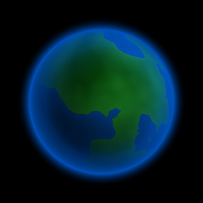
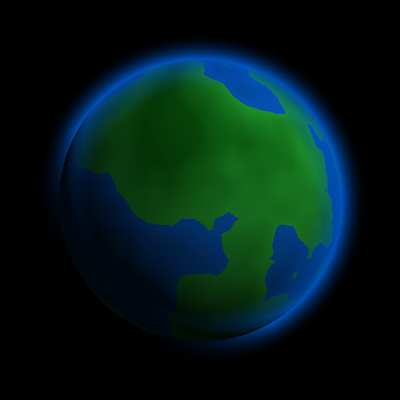
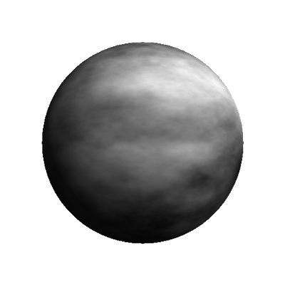
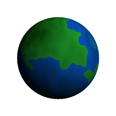
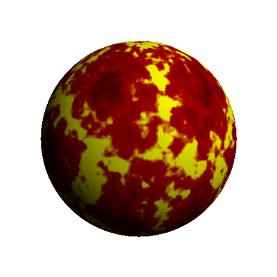
This is part two of my series of posts detailing the rendering of planets in War Worlds. Last time, we started rendering a basic sphere using a very simple ray-tracer. This time, we're going to start work on texturing that sphere.

We're really just laying the ground-work here, getting ready for things to come. In particular, we're going to come up with a way to generate what's known as a delaunay triangulation of random points, and the corresponding Voronoi diagram. Why, you ask? Well, that will all become clear in the next part :-)

Point Cloud

First of all, to generate a delauny triangulation, you need a "point cloud" -- a square of randomly-generate points. The most obvious way to generate such a set of random points is just to generate random x- and y- coordinates. In fact, here's some code that does just that:

PointCloud pc = new PointCloud();

int numPoints = 200; // or some number...
Random rand = new Random();
for (int i = 0; i < numPoints; i++) {
    Vector2 p = new Vector2(rand.nextDouble(), rand.nextDouble());
    pc.mPoints.add(p);
}

This code uses my helper Vector2 class to hold an instance of a 2D-point and my PointCloud class that holds a collection of Vector2 points. I define my point cloud to only contain points between (0,0) and (1,1) which simplifies things a little later on.

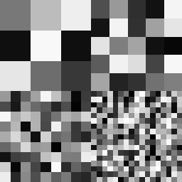
But this produces... unsatisfying results:

As you can see, the points are kind of clumped together and they don't look very attractive. You may remember a post I had a while ago where I was talking about exactly this problem with the randomly-generated starfield. You may also remember that I solved the problem using a Poisson distribution function. Well, the same thing can be used here to generate some nice-looking, random-but-approximately-evenly-distributed points:

The code to generate a poisson distribution is actually fairly simple, conceptually. You start with a single point, then you generate a whole bunch of points around that point a random distance and rotation away. Then you throw out all the ones that are too close together, and you keep generating new points from each of the ones you just generated. Here it is in code form:

// start with a single random point
List<Vector2> unprocessed = new ArrayList<Vector2>();
unprocessed.add(new Vector2(mRand.nextDouble(), mRand.nextDouble()));

// we want minDistance to be small when density is high and big when
// density is small.
double minDistance = 0.001 + ((1.0 / mDensity) * 0.03);

// packing is how many points around each point we'll test for a new
// location. A high randomness means we'll have a low number (more
// random) and a low randomness means a high number (more uniform).
int packing = 10 + (int) ((1.0 - mRandomness) * 90);

while (!unprocessed.isEmpty()) {
    // get a random point from the unprocessed list
    int index = mRand.nextInt(unprocessed.size());
    Vector2 point = unprocessed.get(index);
    unprocessed.remove(index);

    // if there's another point too close to this one, drop it
    if (inNeighbourhood(pc.mPoints, point, minDistance)) {
        continue;
    }

    // otherwise, this is a good one, add it to the final list
    pc.mPoints.add(point);

    // now generate a bunch of points around this one...
    for (int i = 0; i < packing; i++) {
        Vector2 newPoint = generatePointAround(point, minDistance);
        if (newPoint.x < 0.0 || newPoint.x > 1.0)
            continue;
        if (newPoint.y < 0.0 || newPoint.y > 1.0)
            continue;

        unprocessed.add(newPoint);
    }
}

As you can see, we start with a single random point, add it to an "unprocessed" list. Then, for each point in the list we make sure no other points in the "final" list are too close to it (as defined by the minDistance parameter). inNeighbourhood is a simple O(n) function like so:

private boolean inNeighbourhood(List<Vector2> points, Vector2 point,
                                double minDistance) {
    for (Vector2 otherPoint : points) {
        if (point.distanceTo(otherPoint) < minDistance) {
            return true;
        }
    }

    return false;
}

Yeah, not very efficient. Once we're happy with the point, we add it to the PointCloud, and then generate a bunch of points around it using generatePointAround. A quick check that the newly generate points are in the valid range and we add them to the "unprocessed" collection.

private Vector2 generatePointAround(Vector2 point, double minDistance) {
    double radius = minDistance * (1.0 + mRand.nextDouble());
    double angle = 2.0 * Math.PI * mRand.nextDouble();

    return new Vector2(point.x + radius * Math.cos(angle),
                        point.y + radius * Math.sin(angle));
}

The new points are generated radius distance from the existing point (you can see radius will range from minDistance to minDistance * 2), and random direction from 0 to 2π.

The parameters mDensity and mRandomness are parameters I can tune to generate a different set of points. Here's another set of points, where I've turned the density up (and hence minDistance down):

Delaunay Triangulation

So we have our nice point cloud, next we want to triangulate that into a series of triangles. For that, we use a technique called the Delaunay triangulation. While researching this, I learnt a new word today: circumcircle. Basically, the circumcircle of a collection of points is a circle that touches each of the points. For a triangle, three points, there's guaranteed to be exactly one circumcircle (for more points, it may be impossible to circumcircle all of the points).

I'll admit that I pretty much just took the code below directly from here, rather than working it out on my own. If you really want to work out how to calculate the circumscribed circle of a triangle, the wikipedia page on the subject describes how it works pretty succinctly.

private void calculateCircumscribedCircle() {
    final double EPSILON = 0.000000001;

    if (Math.abs(v1.y - v2.y) < EPSILON && Math.abs(v2.y - v3.y) < EPSILON) {
        // the points are coincident, we can't do this...
        return;
    }

    double xc, yc;
    if (Math.abs(v2.y - v1.y) < EPSILON) {
        final double m = - (v3.x - v2.x) / (v3.y - v2.y);
        final double mx = (v2.x + v3.x) / 2.0;
        final double my = (v2.y + v3.y) / 2.0;
        xc = (v2.x + v1.x) / 2.0;
        yc = m * (xc - mx) + my;
    } else if (Math.abs(v3.y - v2.y) < EPSILON ) {
        final double m = - (v2.x - v1.x) / (v2.y - v1.y);
        final double mx = (v1.x + v2.x) / 2.0;
        final double my = (v1.y + v2.y) / 2.0;
        xc = (v3.x + v2.x) / 2.0;
        yc = m * (xc - mx) + my; 
    } else {
        final double m1 = - (v2.x - v1.x) / (v2.y - v1.y);
        final double m2 = - (v3.x - v2.x) / (v3.y - v2.y);
        final double mx1 = (v1.x + v2.x) / 2.0;
        final double mx2 = (v2.x + v3.x) / 2.0;
        final double my1 = (v1.y + v2.y) / 2.0;
        final double my2 = (v2.y + v3.y) / 2.0;
        xc = (m1 * mx1 - m2 * mx2 + my2 - my1) / (m1 - m2);
        yc = m1 * (xc - mx1) + my1;
    }

    centre = new Vector2(xc, yc);
    radius = centre.distanceTo(v2);
}

You can see at the end of this function, we get the centre and radius of the circumscribed circle of a triangle defined by v1, v2 and v3. So how do we use this to generate a delaunay triangulation? The easiest way to generate a delaunay triangulation is to start with an already-generated triangulation, and add vertices to it one by one. So let's say we have the following triangulation, and we're trying to add the red dot in the middle:

The first thing we need to do is gather all of the triangles whose circumcircle encloses the new point. You can visualize this like so:

You can see the point is enclosed by two of the circumcircles. So these two triangles are the ones we're interested in. We need to take these two triangles out of the triangulation, then we need to separate out all of the "outside" edges. This is actually pretty simple: the outside edges are all of the ones that are not doubled-up. This picture can hopefully visualize that:

So we remove the double-up edges and we're left only with "outside" edges of this polygon. Simple connect each edge to the new point and we're done:

The only question is, if you've just got a point cloud, how do you start out? Easy: create two "super triangles" that enclose all of the points in your point cloud and start adding points from there. Once you're done, you need to remove all triangles which share an edge with the "super triangle".

Here's the algorithm in code form:

public void generate() {
    ArrayList<Triangle> triangles = new ArrayList<Triangle>();
    List<Vector2> points = mPointCloud.getPoints();

    // first, create a "super triangle" that encompasses the whole point
    // cloud.
    List<Triangle> superTriangles = createSuperTriangles(points, triangles);

    // go through the vertices and add them...
    for (int i = 0; i < points.size(); i++) {
        addVertex(points, triangles, i);
    }

    // now go through the triangles and copy any that don't share a vertex
    // with the super triangles to the final array
    mTriangles = new ArrayList<Triangle>();
    for (Triangle t : triangles) {
        boolean sharesVertex = false;
        for (Triangle st : superTriangles) {
            if (st.shareVertex(t)) {
                sharesVertex = true;
                break;
            }
        }

        if (!sharesVertex) {
            mTriangles.add(t);
        }
    }
}

I hope createSuperTriangles is obvious, so I won't go into detail. Basically, I just create two triangles that wrap the whole set of points (which is easy for me because I know my points all lie in the range (0,0) to (1,1). The addVertex method is the heart of the algorithm:

private void addVertex(List<Vector2> points, List<Triangle> triangles,
                       int vIndex) {
    Vector2 pt = points.get(vIndex);

    // extract all triangles in the circumscribed circle around this point
    ArrayList<Triangle> circumscribedTriangles = new ArrayList<Triangle>();
    for (Triangle t : triangles) {
        if (t.isInCircumscribedCircle(pt)) {
            circumscribedTriangles.add(t);
        }
    }
    triangles.removeAll(circumscribedTriangles);

    // create an edge buffer of all edges in those triangles
    ArrayList<Edge> edgeBuffer = new ArrayList<Edge>();
    for (Triangle t : circumscribedTriangles) {
        edgeBuffer.add(new Edge(t.a, t.b));
        edgeBuffer.add(new Edge(t.b, t.c));
        edgeBuffer.add(new Edge(t.c, t.a));
    }

    // extract all of the edges that aren't doubled-up
    ArrayList<Edge> uniqueEdges = new ArrayList<Edge>();
    for (Edge e : edgeBuffer) {
        if (!e.isIn(edgeBuffer)) {
            uniqueEdges.add(e);
        }
    }

    // now add triangles using the unique edges and the new point!
    for (Edge e : uniqueEdges) {
        triangles.add(new Triangle(points, vIndex, e.a, e.b));
    }
}

So we're using my Triangle and Edge helper classes. These two classes contain indices in the points collection of their vertices. The Triangle.isInCircumscribedCircle() method uses the centre and radius of the circumscribed circle I calculated above.

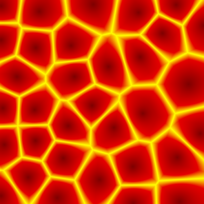
So once all of that is done, I can generate images such as this:

Voronoi diagrams

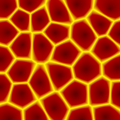
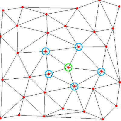
Voronoi diagrams are simply a different representation of the same data you get from the delaunay triangulation. A voronoi diagram is calculated by taking a point from the point cloud, then looking at each triangle attached to that point. Connect up the circumcircles of each of those triangles and you've got one cell of the voronoi diagram. Here's a picture:

The green lines are the delaunay triangulation, the blue lines are the voronoi diagram. In my code, the only special thing I store for the Voronoi diagram is a mapping of points to the triangles that share that point as a vertex. Then it's a matter of drawing the Voronoi diagram like so:

public void renderVoroni(Image img, Colour c) {
    for (Vector2 pt : mPointCloud.getPoints()) {
        List<Triangle> triangles = mPointCloudToTriangles.get(pt);

        for (int i = 0; i < triangles.size() - 1; i++) {
            img.drawLine(c, triangles.get(i).centre,
                         triangles.get(i+1).centre);
        }
        img.drawLine(c, triangles.get(0).centre,
                     triangles.get(triangles.size() - 1).centre);
    }
}

The main tricky part about this code is that it assumes the triangles are sorted in clockwise (or counter-clockwise) order. That is, drawing from triangles[0] to triangles[1] to triangles[2] etc will draw the outline of the cell. That just took a bit of finagling of the triangles when I added them to the mapping, but nothing too complicated. In fact, for normal usage the finagling isn't really needed, you can just take the triangles in any old order, it's only needed to get the display correct.

Tweaking the parameters

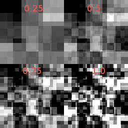
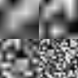
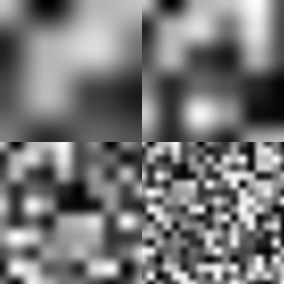
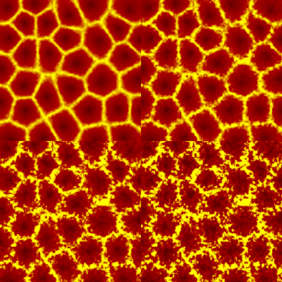
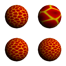
And this brings us back to the little test application I was working on yesterday. I've added a few more controls so that now I can generate all the images from this post on-demand. I can tweak the various parameters and see just how it all turns out. Here's some examples:

Different parameters:

You can see even with the maximum "density", the total elapsed time is still under a quarter of a second. That's not great, but in reality I expect the top screenshot (with density set to 0.5) to be much more useful. Another thing I've noticed is that setting the "randomness" higher (e.g. 1.0) doesn't make much difference to the overall quality but has significantly better performance.

In any case, the place to optimize here is obviously the point cloud generation -- the triangulation code, for all it's inefficiency, is still much faster.

One other point, there's something funny going on at the edges of my voronoi diagrams. It looks like this is related to the fact that points at the edges have nicely enclosing triangles. It's not a huge problem, since I can hide the edges of my texture maps in the game, but maybe something I should look into if I get a chance.

Next time

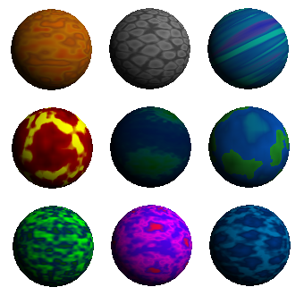
Coming up next time, we'll look at what we can actually do with voronoi diagrams. For some hints, you might want to check Google image search to see what others have been doing.

Series Index

Here are some quick links to the rest of this series:

• Part 1 (Diffuse lighting)
• Part 2 (Voronoi Diagrams and Delaunay Triangulation) (this part)
• Part 3 (Texture Mapping)
• Part 4 (Perlin Noise)
• Part 5 (Atmosphere and Parameterization)
• Appendix A (Performance Tuning)